Drawing Genealogy Graphs. Part 3: Genealogy Graph Positioning

Intro

This is the third post in a series about building and rendering genealogy graphs. You can see all posts in the series here: /tags#drawing-genealogy-graphs-series.

In the first post, I described the Reingold-Tilford algorithm for positioning tree nodes (calculating (x; y) for each tree node).

In the second post, I described genealogy graph interactivity and how it works in the Grafily plugin.

In the first post, I said that trees, as a data structure for representing relatives, are inconvenient because they simply do not allow you to see siblings of ancestors or parallel families. So, graphs. What's with them? We have a graph representing relationships between families. This graph can be huge and of any form. How can we calculate each node's coordinates to render this graph? In this post, I will try to answer this question and explain my thoughts about it.

Oh, one more thing:

Reingold-Tilford++

My first intuitive approach was to improve the Reingold-Tilford algorithm. Its original version supports only trees. But I wanted to adapt it to graphs and develop a universal algorithm for positioning graph nodes. Surprisingly, I had some (partial) success. I was able to render such graphs:

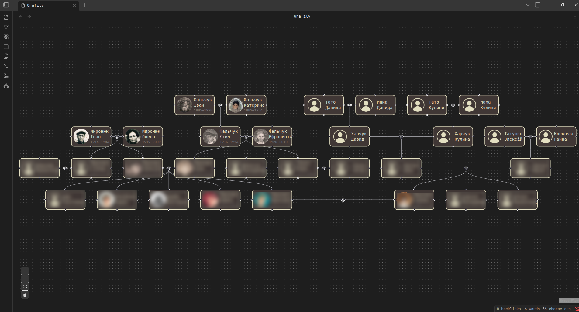
(The screenshot above is around 8 months old. At the moment of writing this post, the plugin UI has changed a lot)

How did I do it? Let me try to explain quickly. First, you need to understand how the original Reingold-Tilford algorithm works. I already explained it in my blog here: Drawing Genealogy Graphs. Part 1: Tree Drawing Using Reingold-Tilford Algorithm.

The Reingold-Tilford algorithm works because of two things:

• The Reingold-Tilford Algorithm uses a depth-first tree traversal. This means that when we calculate the node preX, mod, and shift values, we already have them for all child nodes.
• The node traversal order is fixed. When we calculate the node x coordinate, all child nodes and all nodes to the left of the current node are already centered, and we can calculate the current node properties (preX, mod, and shift).

Overall, I could reuse the preX, mod, and shift parameters and apply them to a graph. I only need to follow the two requirements above.

And I did it: https://github.com/TheBestTvarynka/grafily/pull/1/changes.

1. I defined an unambiguous way to walk through the graph.
2. I simplified the task: I decided to join siblings into one unit (I called it SiblingsUnit). Instead of centering many nodes, the algorithm centers sibling units.

Let's look at the image below:

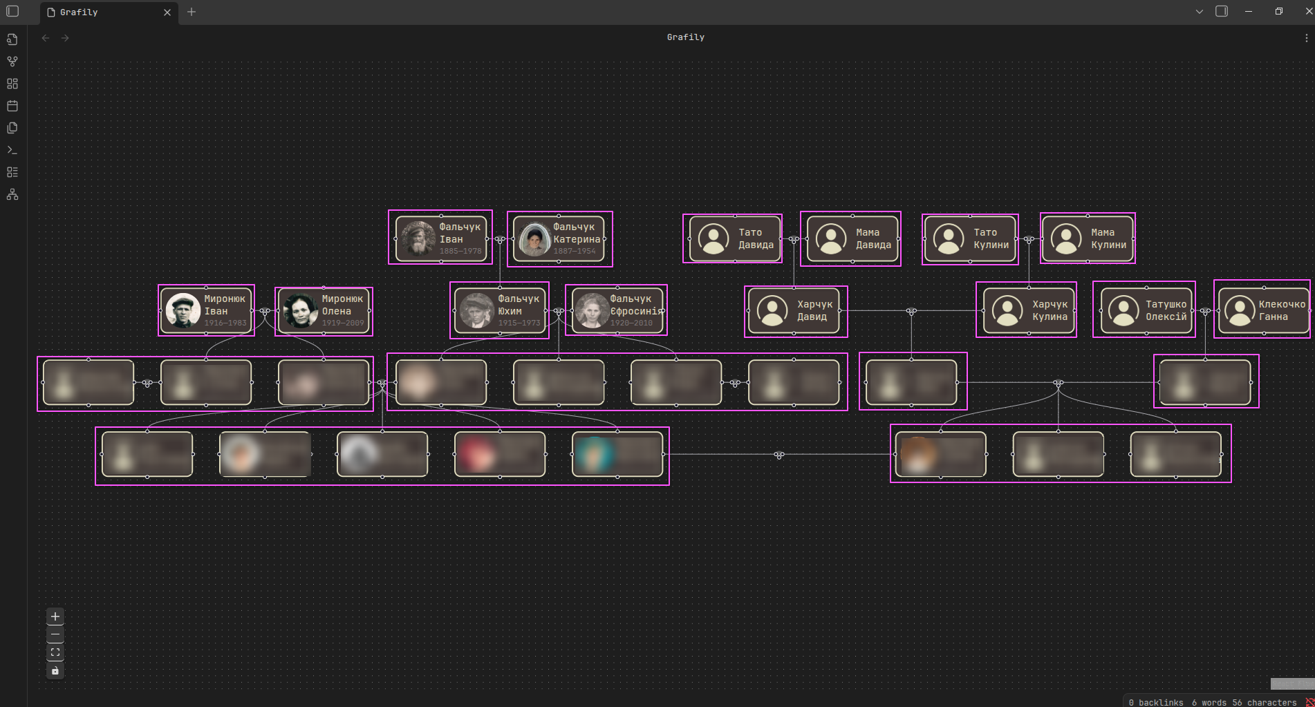
Instead of centering nodes, the algorithm centers purple blocks (sibling units). The algorithm reuses the same preX, mod, and shift parameters but applies them to sibling units instead of nodes. Now let's see the traversal order:

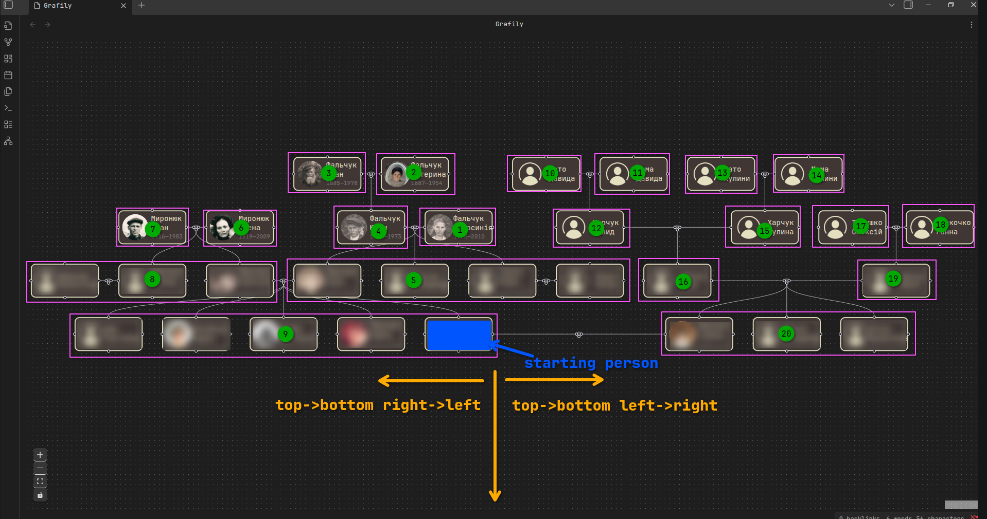
There is always a starting person. Starting from the starting person (😆 🤣), the algorithm first calculates coordinates for the left half of the graph, then for the right. It uses depth-first search: it starts at the topmost rightmost node of the left half and moves to the left and to the bottom. Pay attention to the numbers inside sibling units. These numbers show the order of x coordinate calculation for the sibling unit. At the moment when we calculate the parameters of unit 4, we already know the parameters of unit 3 and unit 2. When calculating the parameters of unit 20, it already knows the parameters of units 16 and 19.

Note that in the left half it visits the rightmost nodes first (right to left), and in the right half it visits the leftmost nodes first (left to right).

That way, I guaranteed a depth-first traversal and an unambiguous way to walk through the graph. Every unit knows parameters of units to the top of it and to the left or right of it.

So, what's the problem? Why did I discard this approach?

This is a problem. In reality, genealogy graphs are way more complex. For example, the described approach does not allow unambiguous traversal of graphs where genealogy lines are expanded to the top and bottom many times. Bleh, it sounds complex 😵‍💫 🥴. It's much easier to show an example:

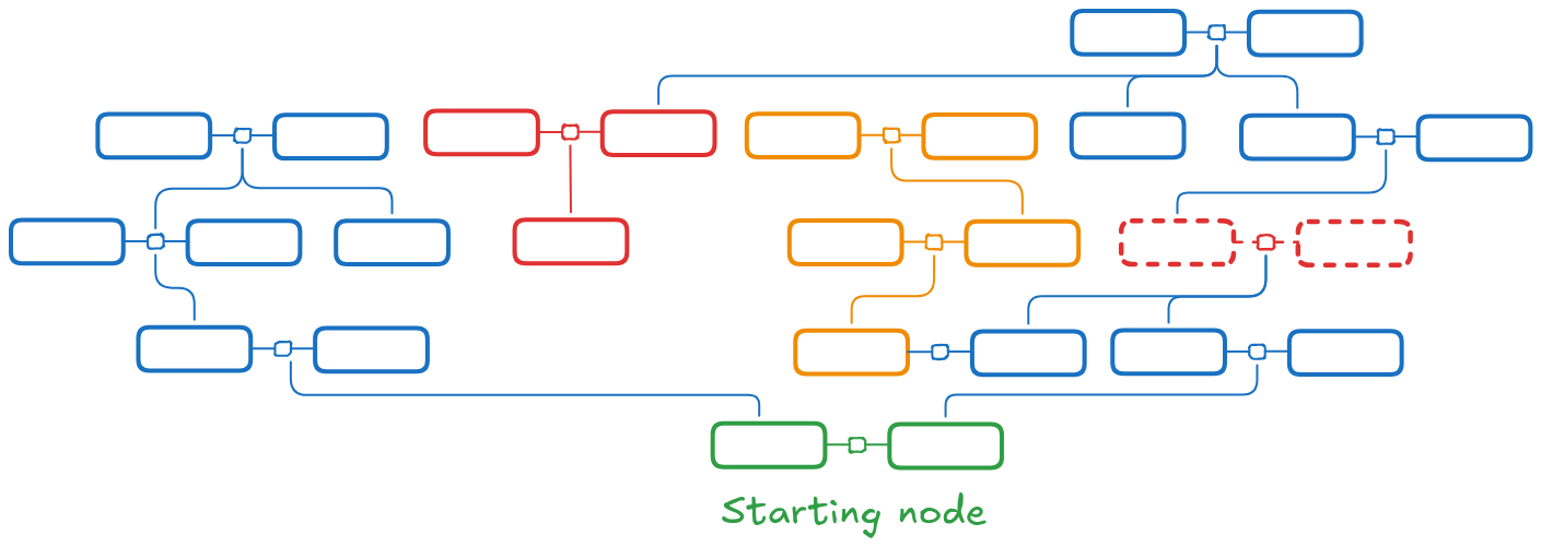
To find coordinates for orange nodes, the algorithm needs the coordinates for red solid nodes. But the algorithm calculates the red solid nodes' coordinates only when it enters the red dashed nodes. But the algorithm cannot enter the red dashed nodes until it finishes with the orange ones. We have a contradiction here: one node depends on another, and the other depends on the first. There is no unambiguous way to resolve this 😵‍💫.

Overall, I can create a special version of depth-first search especially for that case, but it will not work for any kind of graph. So, I wrapped up this approach and started searching for another one.

Brandes-Köpf

Fast enough, I found the Brandes-Köpf algorithm. It was introduced in the Fast and Simple Horizontal Coordinate Assignment paper. It says simle, but do not trust it. My experience says that there are no easy papers to read 🙃.

I spent a few evenings exploring it. It looked like the right call. I decided to try it.

I won't explain in detail how it works. There are two great sources you can read to understand it:

• Fast and Simple Horizontal Coordinate Assignment paper.
• Erratum: Fast and Simple Horizontal Coordinate Assignment paper. It described an improved version of the BK algorithm.

In short, the BK algorithm created a vertical alignment for nodes (blocks) from top to bottom or bottom to top, then grouped them into polygons (classes) from left to right or right to left (horizontal compaction). Classes do not touch and have a defined minimal space between them. For example, below is an image from the paper that illustrates top-to-bottom vertical alignment and right-to-left horizontal compaction (the image below is taken from the paper):

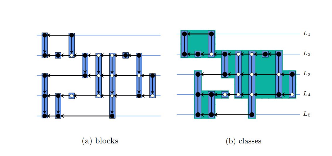
Graph edges are omitted. The arrows in the image above show the traversal order for each class.

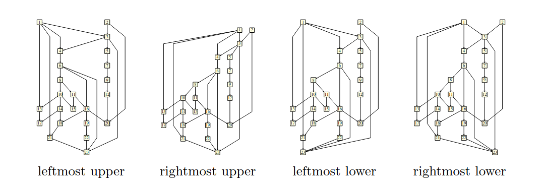
Run the vertical alignment and horizontal compaction steps 4 times (each time you change direction), calculate the average x coordinate for each node, and then produce the final result. In reality, you will calculate an average for each node based on the four previously obtained layouts (the image below is also taken from the paper):

I hope I fed your curiosity 😅. To understand the algorithm completely, you'll definitely need to read the papers carefully.

I did not want to implement it from scratch. I decided to look for an open-source implementation. I didn't find a generic enough implementation to suit my needs. But I found a very good open-source implementation of the Brandes-Köpf algorithm inside the dagree project: github/dagrejs/dagre/2595d05a0f/lib/position/bk.js. Back then I took that algorithm, rewrote it in TypeScript, and adapted it to my case. Soon after, the dagree project also rewrote it in TS. But I kept my implementation because it was already adapted and worked well.

I loaded a few tests, and it looked like the right call. I was pleased by the result:

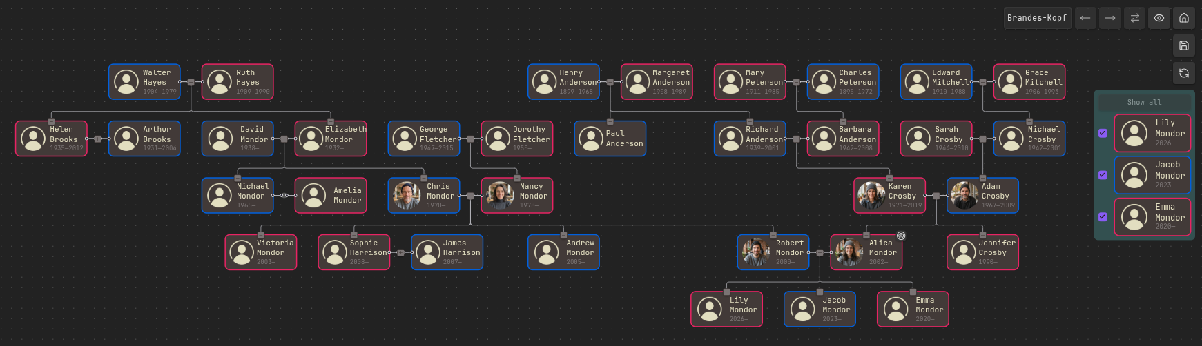
Since there is a third option, you may have already guessed that this is not enough. And you are right. In some cases, the Brandes-Köpf approach produces very poor layouts. Just look:

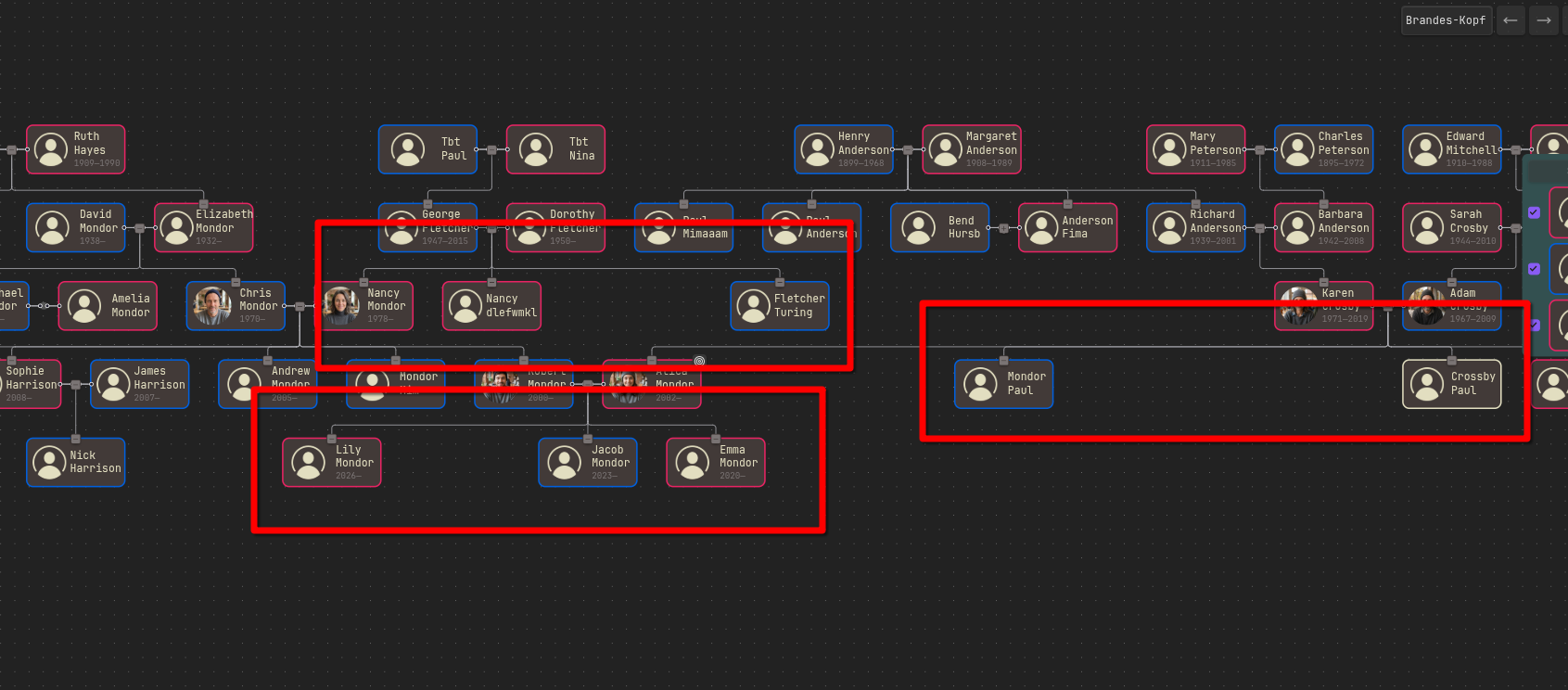
You can clearly see the vertical alignment and when it doesn't work well. That extra space between sibling nodes comes from nodes belonging to different classes (the horizontal compaction step in the Brandes-Köpf algorithm). At first, I thought that this was a rare case and I would eventually get used to it. Unfortunately, I saw it too often and did not get used to it. So, I decided to look for an alternate approach.

Quadratic programming

I spent many hours trying to adapt an algorithm I knew. I made many attempts to find an existing one. Eventually, I gave up and decided to go all-vibe.

The LLM suggested several approaches to improve the layout calculation. There were Quadratic Programming (QP), physics simulation (edges are rubber and pull nodes), etc. The QP was the easiest one to start with. By easiest, I mean the least code to generate and integrate into the existing system. Physics simulation also looks like overkill for such a small problem.

In general, there is a certain function (math equation) that defines the layout (edge lengths or nodes' x-coordinates relative to other nodes). The unified solver then tried to solve that equation. I know nothing about QP, and I went all in with vibe-coding.

First, I built a test playground for testing graph node-positioning algorithms: github/TheBestTvarynka/graph-layout-playground. Experimenting in the grafily repo was inconvenient because I wanted an easy way to inject a test graph and see its layout. Then, I comprehensively described all my requirements for the desired graph layout and node positions. Then I added 3-4 test graphs with different complexity and structure. And finally asked Claude Code (CC) to implement a QP-based layout algorithm.

Honestly, it did a great job, and I really liked it. The resulting graph layout looks better than all my previous tries, almost from the first try. I added more tests and more instructions. CC has improved the code, and I was finally satisfied with the result.

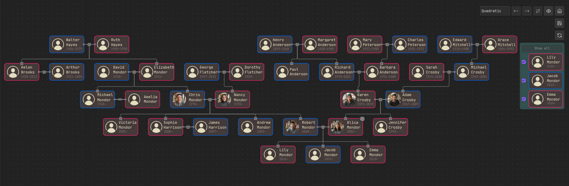
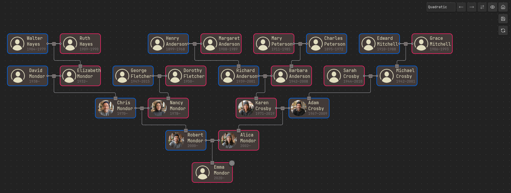
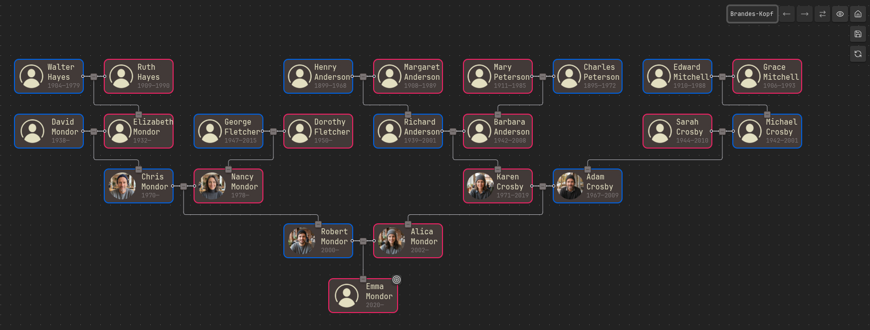
Of course, the final layout algorithm is not perfect either. There is no perfect positioning algorithm. The current one is good enough for 95% of cases. For the remaining 5%, I recommend using the Brandes-Köpf algorithm.

QP	BK

From the comparison above, you can see that the QP-based approach produces more compact and prettier graph layouts. As I said above, the QP-based algorithm works better in 95% of cases (from my experience). When the graph starts looking more like a simple tree, the BK algorithm will be better:

QP	BK

Outro

At the moment, I am fully satisfied with the Grafily graph rendering. Using the Brandes-Köpf and Quadratic algorithms, I can get readable, pretty graphs.

The Grafily plugin keeps, and will keep, both the Brandes-Köpf and Quadratic algorithms. The user can switch between them at any time.

References

1. Brandes-Köpf approach implementation.
2. The Dagre project on GitHub.
3. Fast and Simple Horizontal Coordinate Assignment (paper).
4. QP-based approach implementation.